Symbolic Computing

Symbolic computing allows you to use a computer to do all the algebra you might otherwise do by hand.

SymPy is a popular package for symbolic computing.

conda install sympy

import sympy as sym
import math
import numpy as np

A good place to start is the SymPy tutorial

Let’s compare how sympy evaluates sqrt vs. math

print(math.sqrt(8))
print(np.sqrt(8))

2.8284271247461903
2.8284271247461903

sym.sqrt(8)

\[\displaystyle 2 \sqrt{2}\]

Note that jupyter notebooks render the output nicely.

the math package gives a floating point approximation to \(\sqrt{8}\), whereas sympy simplifies the expression by removing any divisors that are perfect squares.

a = sym.sqrt(8)
print(a)
type(a)

2*sqrt(2)

sympy.core.mul.Mul

Algebraic Expressions

Symbolic computing is particularly useful for manipulating algebraic expressions.

from sympy import symbols, expand, factor

You can build expressions using symbols:

x, y = symbols('x y')
expr = 2*x + y
expr

\[\displaystyle 2 x + y\]

Let’s say we forgot how to mulitply monomials

a, b, c, d = symbols('a b c d')
x, y = symbols('x, y')
ex1 = a*x + b
ex2 = c*x + d
ex1 * ex2

\[\displaystyle \left(a x + b\right) \left(c x + d\right)\]

we can expand an expression by multiplying everything out and combining like terms:

ex = expand(ex1 * ex2)
ex

\[\displaystyle a c x^{2} + a d x + b c x + b d\]

We can also factor an expression that has been expanded:

factor(ex)

\[\displaystyle \left(a x + b\right) \left(c x + d\right)\]

You can substitute values (or other symbols) for symbols:

ex.subs([(a, 1), (b, 2), (c, 3), (d, y)])

\[\displaystyle 3 x^{2} + x y + 6 x + 2 y\]

ex_sub = ex.subs([(a, 1), (b, 2), (c, 2), (d, 3)])
ex_sub

\[\displaystyle 2 x^{2} + 7 x + 6\]

You can evaluate expressions numerically:

ex_sub.evalf(subs={x: 0.1})

\[\displaystyle 6.72\]

SymPy uses arbitrary precision arithmetic. The default precision is 10 decimal digits (between single and double precision), but you can increase the precision in evalf

sym.pi.evalf()

\[\displaystyle 3.14159265358979\]

sym.pi.evalf(100)

\[\displaystyle 3.141592653589793238462643383279502884197169399375105820974944592307816406286208998628034825342117068\]

Symbolic Mathematics

Sympy supports just about everything you might have learned in courses on algebra and calculus (and more)

import sympy as sym

Differentiation

expr = sym.sin(x)
print(expr)
print(sym.diff(expr)) # symbolic differentiation w.r.t x

sin(x)
cos(x)

expr = x * y
sym.diff(expr, x) # differentiate w.r.t. x

\[\displaystyle y\]

Integration

expr = sym.sin(x)
print(expr)
print(sym.integrate(expr, x)) # indefinite integral w.r.t x

sin(x)
-cos(x)

the sympy variable oo (two o symbols) is used to represent \(\infty\)

from sympy import oo
expr = sym.exp(-(x**2))
sym.integrate(expr, (x, -oo, oo)) # integration with limits

\[\displaystyle \sqrt{\pi}\]

sym.integrate(expr, (x, -1, 1))

\[\displaystyle \sqrt{\pi} \operatorname{erf}{\left(1 \right)}\]

Limits

You can compute limits. For example: \begin{equation} \lim_{x\to 0} \frac{\sin(x)}{x} \end{equation}

sym.limit(sym.sin(x)/x, x, 0) # limit as x \to 0

\[\displaystyle 1\]

Roots

You can compute roots of functions using solve (i.e. we solve the system f(x) = 0 for x)

sym.solve(x**2 - 3, x)

[-sqrt(3), sqrt(3)]

Symbolic to Numerical Functions

You can turn sympy functions into lambda functions that are compatible with numpy using lambdify:

f = sym.sin(x)
g = sym.lambdify(x, f, 'numpy')
g(np.array(np.linspace(0,1,10)))

array([0.        , 0.11088263, 0.22039774, 0.3271947 , 0.42995636,
       0.52741539, 0.6183698 , 0.70169788, 0.77637192, 0.84147098])

Plotting Functions

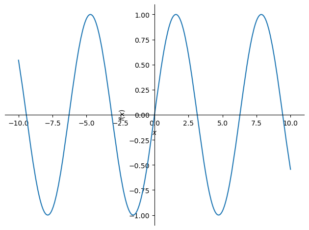
You can plot a symbolic function using the sympy plot function

f = sym.sin(x)
sym.plot(f)

<sympy.plotting.plot.Plot at 0x7f91e02a3f10>

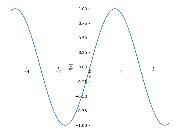
you can change the domain using a tuple with the variable and lower and upper bounds

sym.plot(f, (x, -5,5))

<sympy.plotting.plot.Plot at 0x7f91de74bd50>

There are a variety of keyword arguments you can use for formatting as well. See help(sym.plot) for more information.

Exercises

Use sympy to compute solutions to answer the following questions

1. What is \(\int_{1}^{\infty} x^{-2}\, dx\)?

2. Find a value of x where sin(x) = cos(x)

sym.integrate((x)**(-2), (x, 1, oo))

\[\displaystyle 1\]

from sympy.solvers import solve
from sympy import *
x = Symbol('x')
solve(sin(x)-cos(x),x) 

[pi/4]