Scipy stats package

A variety of functionality for dealing with random numbers can be found in the scipy.stats package.

• scipy.stats tutorial

• scipy.stats reference

from scipy import stats
import matplotlib.pyplot as plt
import numpy as np

Distributions

There are over 100 continuous (univariate) distributions and about 15 discrete distributions provided by scipy

• continuous distributions

• discrete distributions

To avoid confusion with a norm in linear algebra we’ll import stats.norm as normal

from scipy.stats import norm as normal

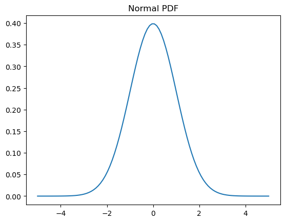
A normal distribution with mean \(\mu\) and variance \(\sigma^2\) has a probability density function \begin{equation} \frac{1}{\sigma \sqrt{2\pi}} e^{-(x-\mu)^2 / 2\sigma^2} \end{equation}

# bounds of the distribution accessed using fields a and b
normal.a, normal.b

(-inf, inf)

# mean and variance
normal.mean(), normal.var()

(0.0, 1.0)

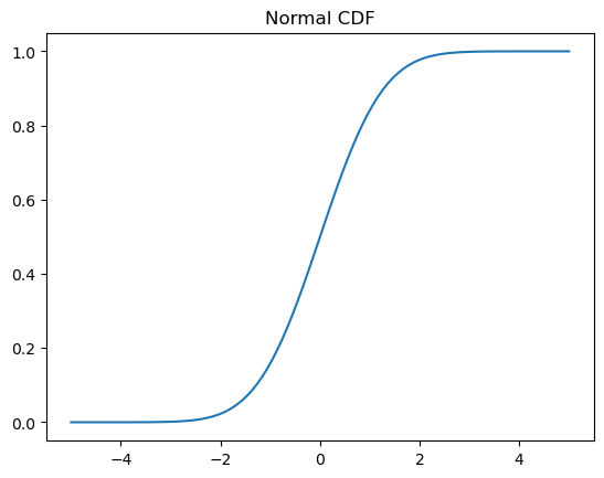
# Cumulative distribution function (CDF)
x = np.linspace(-5,5,100)
y = normal.cdf(x)
plt.plot(x, y)
plt.title('Normal CDF');

# Probability density function (PDF)
x = np.linspace(-5,5,100)
y = normal.pdf(x)
plt.plot(x, y)
plt.title('Normal PDF');

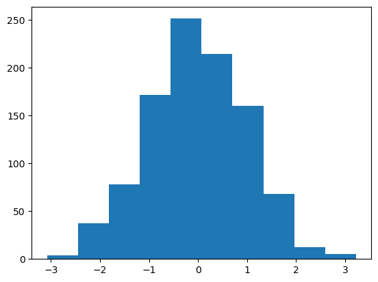
You can sample from a distribution using the rvs method (random variates)

X = normal.rvs(size=1000)
plt.hist(X);

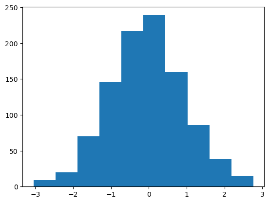
You can set a global random state using np.random.seed or by passing in a random_state argument to rvs

X = normal.rvs(size=1000, random_state=0)
plt.hist(X);

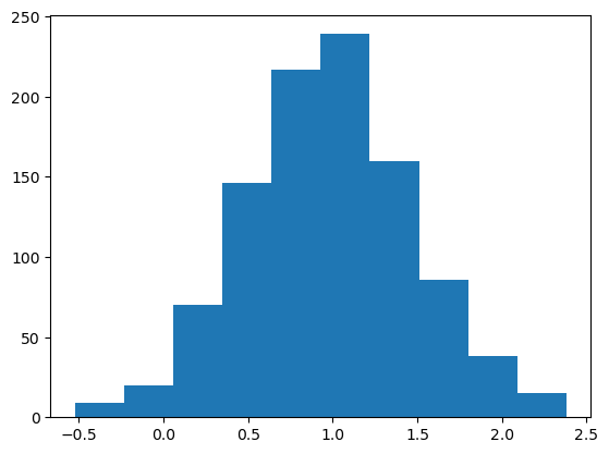
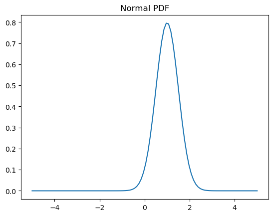
To shift and scale any distribution, you can use the loc and scale keyword arguments

X = normal.rvs(size=1000, random_state=0, loc=1.0, scale=0.5)
plt.hist(X);

# Probability density function (PDF)
x = np.linspace(-5,5,100)
y = normal.pdf(x, loc=1.0, scale=0.5)
plt.plot(x, y)
plt.title('Normal PDF');

You can also “freeze” a distribution so you don’t need to keep passing in the parameters

dist = normal(loc=1.0, scale=0.5)
X = dist.rvs(size=1000, random_state=0)
plt.hist(X);

Example: The Laplace Distribution

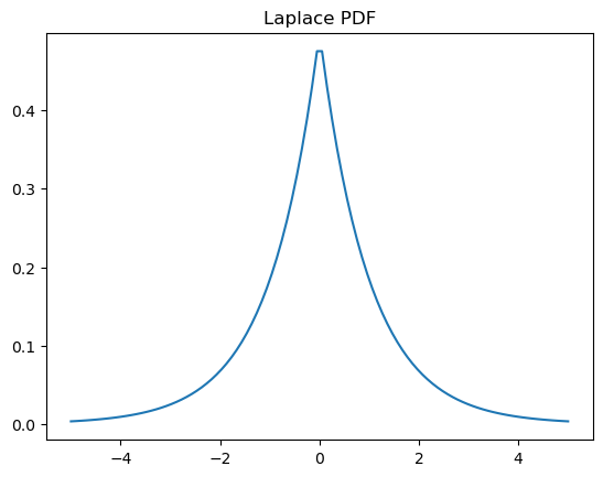
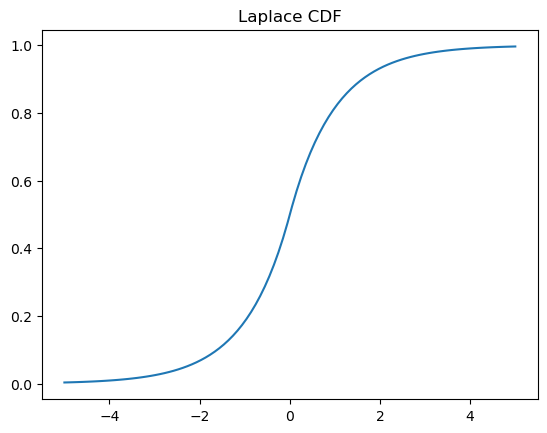
We’ll review some of the methods we saw above on the Laplace distribution, which has a PDF \begin{equation} \frac{1}{2}e^{-|x|} \end{equation}

from scipy.stats import laplace

x = np.linspace(-5,5,100)
y = laplace.pdf(x)
plt.plot(x, y)
plt.title('Laplace PDF');

x = np.linspace(-5,5,100)
y = laplace.cdf(x)
plt.plot(x, y)
plt.title('Laplace CDF');

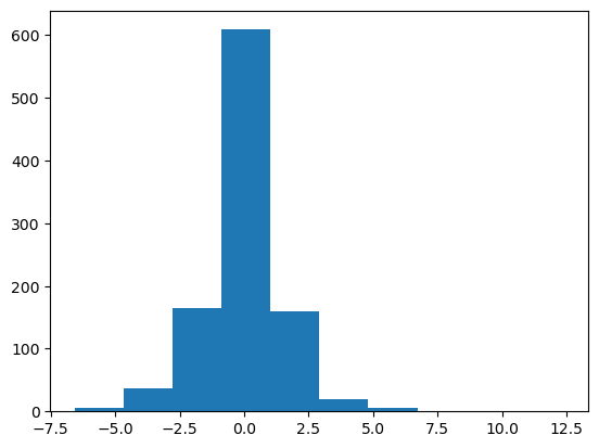
X = laplace.rvs(size=1000)
plt.hist(X);

laplace.a, laplace.b

(-inf, inf)

laplace.mean(), laplace.var()

(0.0, 2.0)

Discrete Distributions

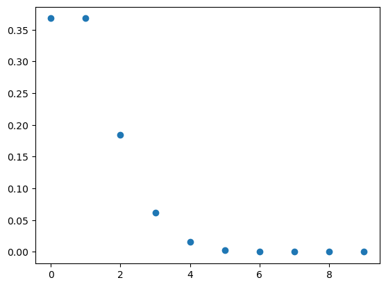
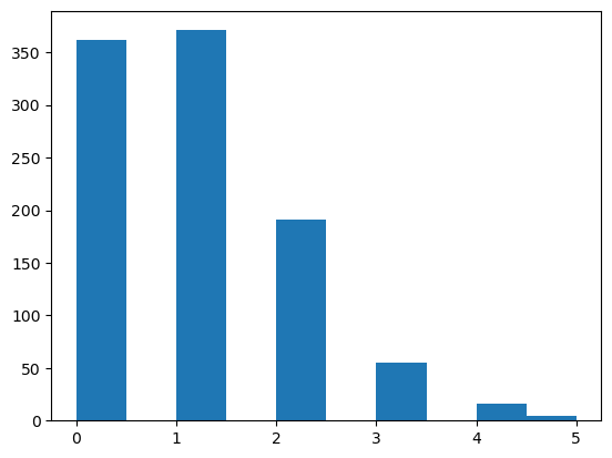
Discrete distributions have many of the same methods as continuous distributions. One notable difference is that they have a probability mass function (PMF) instead of a PDF.

We’ll look at the Poisson distribution as an example

from scipy.stats import poisson
dist = poisson(1) # parameter 1

dist.a, dist.b

(0, inf)

dist.mean(), dist.var()

(1.0, 1.0)

x = np.arange(10)
y = dist.pmf(x)
plt.scatter(x, y);

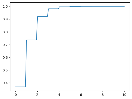
x = np.linspace(0,10, 100)
y = dist.cdf(x)
plt.plot(x, y);

X = dist.rvs(size=1000)
plt.hist(X);

Fitting Parameters

You can fit distributions using maximum likelihood estimates

X = normal.rvs(size=100, random_state=0)

normal.fit_loc_scale(X)

(0.059808015534485, 1.0078822447165796)

Statistical Tests

You can also perform a variety of tests. A list of tests available in scipy available can be found here.

the t-test tests whether the mean of a sample differs significantly from the expected mean

stats.ttest_1samp(X, 0)

TtestResult(statistic=0.5904283402851698, pvalue=0.5562489158694675, df=99)

The p-value is 0.56, so we would expect to see a sample that deviates from the expected mean at least this much in about 56% of experiments. If we’re doing a hypothesis test, we wouldn’t consider this significant unless the p-value were much smaller (e.g. 0.05)

If we want to test whether two samples could have come from the same distribution, we can use a Kolmogorov-Smirnov (KS) 2-sample test

X0 = normal.rvs(size=1000, random_state=0, loc=5)
X1 = normal.rvs(size=1000, random_state=2, loc=5)

stats.ks_2samp(X0, X1)

KstestResult(statistic=0.023, pvalue=0.9542189106778983, statistic_location=5.848821448664333, statistic_sign=-1)

We see that the two samples are very likely to come from the same distribution

X0 = normal.rvs(size=1000, random_state=0)
X1 = laplace.rvs(size=1000, random_state=2)

stats.ks_2samp(X0, X1)

KstestResult(statistic=0.056, pvalue=0.08689937254547132, statistic_location=1.5363770542457977, statistic_sign=1)

When we draw from a different distribution, the p-value is much smaller, indicating that the samples are less likely to have been drawn from the same distribution.

Kernel Density Estimation

We might also want to estimate a continuous PDF from samples, which can be accomplished using a Gaussian kernel density estimator (KDE)

X = np.hstack((laplace.rvs(size=100), normal.rvs(size=100, loc=5)))
plt.hist(X);

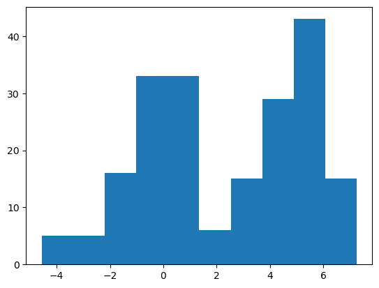
A KDE works by creating a function that is the sum of Gaussians centered at each data point. In Scipy this is implemented as an object which can be called like a function

kde = stats.gaussian_kde(X)
x = np.linspace(-5,10,500)
y = kde(x)
plt.plot(x, y)
plt.title("KDE");

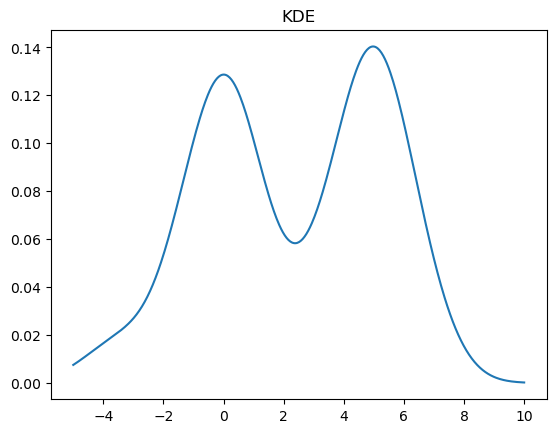
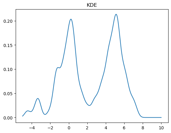
We can change the bandwidth of the Gaussians used in the KDE using the bw_method parameter. You can also pass a function that will set this algorithmically. In the above plot, we see that the peak on the left is a bit smoother than we would expect for the Laplace distribution. We can decrease the bandwidth parameter to make it look sharper:

kde = stats.gaussian_kde(X, bw_method=0.2)
x = np.linspace(-5,10,500)
y = kde(x)
plt.plot(x, y)
plt.title("KDE");

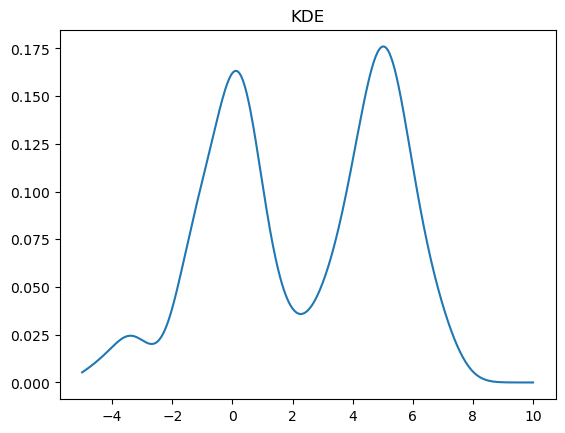
If we set the bandwidth too small, then the KDE will look a bit rough.

kde = stats.gaussian_kde(X, bw_method=0.1)
x = np.linspace(-5,10,500)
y = kde(x)
plt.plot(x, y)
plt.title("KDE");